Antibiotic resistance evolution
DHFR · Trimethoprim selection in E. coli
In this tutorial, we’ll use GraphFLA to explore how mutations in a gene shape bacterial fitness under antibiotic treatment. To see how this works, we’ll build and analyse a nucleotide landscape of the enzyme dihydrofolate reductase (DHFR), then measure its ruggedness, epistasis and navigability.

Download notebook Notebook + data
Run the notebook in Google Colab, or download it to run locally. It downloads its data when no data/ folder is beside it.
1. Setting up
On Google Colab, the cell below installs GraphFLA. In any environment, it also downloads the dataset into a data/ folder next to the notebook if the files are not already there.
We then import GraphFLA for landscape construction and analysis, pandas for working with the data, and NumPy and Matplotlib for the figures.
import sys
from pathlib import Path
from urllib.request import urlretrieve

if "google.colab" in sys.modules:
    %pip install -q graphfla==0.4.0

DATA_URL = "https://raw.githubusercontent.com/COLA-Laboratory/GraphFLA/v0.4.0/tutorials/datasets/data/"
Path("data").mkdir(exist_ok=True)
for name in ["dhfr.csv"]:
    if not Path("data", name).exists():
        urlretrieve(DATA_URL + name, Path("data", name))
from graphfla import analysis
from graphfla.landscape import DNALandscape
import matplotlib.pyplot as plt
import numpy as np
import pandas as pd
2. Loading the dataset
DHFR is an essential metabolic enzyme and the target of the antibiotic trimethoprim. Papkou et al. (2023) used genome editing in Escherichia coli to create all combinations of the nine nucleotides encoding three adjacent amino acids, A26, D27 and L28. This gives 4⁹ = 262,144 genotypes, of which the authors’ archived table contains 261,333 with measured fitness in the presence of trimethoprim.
We’ll maximise this fitness. On the authors’ scale, the wild type GCCGATCTC has fitness 0, and higher values mean better growth under the antibiotic.
| Column | Meaning |
|---|---|
sequence |
Nucleotides at the nine positions, codons 26, 27 and 28 in order. |
fitness |
Fitness relative to the wild type. |
Let’s load the measurements:
df = pd.read_csv("data/dhfr.csv", float_precision="round_trip")
df.head()
Output
/var/folders/cr/vx9vlg4j2_74p6mm66j9hs6r0000gn/T/ipykernel_52850/1354316424.py:1: Pandas4Warning: The 'float_precision' argument is deprecated. Use the default float precision instead.
  df = pd.read_csv("data/dhfr.csv", float_precision="round_trip")
| sequence | fitness | |
|---|---|---|
| 0 | GCCGATCTC | 0.000000 |
| 1 | AAAAAAAAA | -0.733843 |
| 2 | AAAAAAAAC | -0.656973 |
| 3 | AAAAAAAAG | -0.701521 |
| 4 | AAAAAAAAT | -0.708582 |
3. Preparing the inputs
To construct a landscape, GraphFLA needs two aligned inputs:
X: one row per configuration and one column per variable.f: one measured or calculated outcome for each row ofX.
The nucleotide sequence forms X, and fitness forms f. DNALandscape reads each sequence string as nine positions with the alphabet A, C, G and T.
X = df["sequence"]
f = df["fitness"]
X.head()
Output
0    GCCGATCTC
1    AAAAAAAAA
2    AAAAAAAAC
3    AAAAAAAAG
4    AAAAAAAAT
Name: sequence, dtype: str
4. Constructing the landscape
We can use DNALandscape, where neighbouring genotypes differ by a single nucleotide substitution. We set maximize=True because higher fitness is better.
Papkou et al. classified genotypes with fitness below −0.508 as nonfunctional and removed mutational steps between two nonfunctional genotypes before analysing the largest connected network. Setting tau=-0.507774 with filter_mode="both" applies the same rule. With epsilon=0, any fitness difference counts as an improving move, as in the original analysis.
landscape = DNALandscape(maximize=True)
landscape.build_from_data(
    X, f, tau=-0.507774, filter_mode="both", epsilon=0, verbose=False,
)
Output
DNALandscape(maximize=True)
5. Inspecting the landscape
Let’s first look at what we’ve built. Printing the landscape shows its variables, configurations, improving edges and local optima:
print(landscape)
Output
DNALandscape(kind='dna'): 9 variables, 135178 configurations, 324044 edges, 514 local optima
The network keeps 135,178 genotypes, matching the network analysed by Papkou et al. For a closer look at individual genotypes, we can call get_data(). The nine nucleotides appear as pos_0 to pos_8; out_degree counts directly improving moves, and is_lo indicates local-optimum membership.
landscape.get_data().head()
Output
| pos_0 | pos_1 | pos_2 | pos_3 | pos_4 | pos_5 | pos_6 | pos_7 | pos_8 | fitness | in_degree | out_degree | is_lo | |
|---|---|---|---|---|---|---|---|---|---|---|---|---|---|
| 0 | G | C | C | G | A | T | C | T | C | 0.000000 | 12 | 8 | False |
| 1 | A | A | A | A | A | A | A | A | A | -0.733843 | 0 | 1 | False |
| 2 | A | A | A | A | A | A | A | A | C | -0.656973 | 0 | 1 | False |
| 3 | A | A | A | A | A | A | A | A | G | -0.701521 | 0 | 1 | False |
| 4 | A | A | A | A | A | A | A | A | T | -0.708582 | 0 | 1 | False |
We can also summarise the fitness values with pandas:
landscape.get_data()["fitness"].describe()
Output
count    135178.000000
mean         -0.585424
std           0.389963
min          -1.174803
25%          -0.750818
50%          -0.701699
75%          -0.639704
max           1.395792
Name: fitness, dtype: float64
Most genotypes in the network are nonfunctional, with fitness below −0.508. To inspect the fittest genotype, we can use the global-optimum node index:
landscape[landscape.go_index]
Output
{'pos_0': 'A',
 'pos_1': 'A',
 'pos_2': 'G',
 'pos_3': 'G',
 'pos_4': 'A',
 'pos_5': 'A',
 'pos_6': 'A',
 'pos_7': 'T',
 'pos_8': 'G',
 'fitness': np.float64(1.395791684395264),
 'in_degree': 27,
 'out_degree': 0,
 'is_lo': True}
6. Analysing the landscape
Next, we’ll follow three questions in turn: how rugged the landscape is (6.1–6.2), which kinds of epistasis make it so (6.3–6.7), and whether evolution can still reach the best variant (6.8–6.10).
6.1 Number of local optima
We can start with landscape.n_lo. A local optimum, or fitness peak, is a variant without a fitter single-mutant neighbour; each connected neutral plateau of peaks counts once. Many peaks mean that adaptive walks, which accept only fitness-increasing mutations, can end at different variants.
print(f"Number of local optima: {landscape.n_lo}")
Output
Number of local optima: 514
This reproduces the 514 fitness peaks reported by Papkou et al. We can also count the peaks that are fitter than the wild type:
peaks = landscape.get_data(lo_only=True)
print(f"Peaks fitter than the wild type: {(peaks['fitness'] > 0).sum()}")
Output
Peaks fitter than the wild type: 106
6.2 Roughness-to-slope ratio
The peak count shows that the landscape is rugged, but not how far it departs from the simplest case. If every mutation had the same effect in every background, fitness would be additive and the landscape would have a single peak. The roughness-to-slope ratio, introduced by Aita et al. (2000), measures this departure: it fits an additive model and compares the scatter left unexplained with the average size of the mutation effects. Values near zero indicate a nearly additive landscape; larger values indicate a more rugged one.
r_s_ratio() encodes each position relative to a reference nucleotide, so we compare values only when they are calculated in the same way.
roughness_to_slope = analysis.r_s_ratio(landscape)
print(f"Roughness-to-slope ratio: {roughness_to_slope:.4f}")
Output
Roughness-to-slope ratio: 3.3562
6.3 Gamma star
Not every departure from additivity creates peaks. A mutation that is beneficial in every background still leads uphill; multiple peaks can arise only when mutation effects reverse direction between backgrounds, known as sign epistasis. Ferretti et al. (2016) proposed measuring epistasis by how well a mutation’s effect carries over when a second mutation is added to the background. gamma_star() applies this idea to the direction of effects only; we run it in a single process (n_jobs=1), which is fast enough here.
A value of 1 means mutations never switch between beneficial and deleterious; values near zero indicate frequent switches, and negative values indicate that pairs of mutations often reverse each other’s direction (reciprocal sign epistasis).
sign_correlation = analysis.gamma_star(landscape, n_jobs=1)
print(f"Gamma star: {sign_correlation:.4f}")
Output
Gamma star: 0.1417
6.4 Idiosyncratic epistasis
Gamma star records only whether effects change direction. Even when the direction holds, the size of an effect can change from one background to another. Lyons et al. (2020) introduced the idiosyncratic index to measure this variation: it compares the spread of a mutation’s effects across backgrounds with the fitness differences between randomly paired variants. A value of zero means each mutation has the same effect everywhere; a value near one means its effect varies about as much as the difference between two random variants.
global_idiosyncratic_index() averages this index over all mutations. Random pairs are drawn with a fixed seed.
idiosyncrasy = analysis.global_idiosyncratic_index(landscape, seed=42, n_jobs=1)
print(f"Global idiosyncratic index: {idiosyncrasy:.4f}")
Output
Global idiosyncratic index: 0.4593
6.5 Types of epistasis
Gamma star and the idiosyncratic index each reduce epistasis to a single number. classify_epistasis() instead sorts pairs of mutations into types. For each square of four genotypes (the background, two single mutants and the double mutant), it asks how the effect of one mutation changes when the other is present: magnitude epistasis changes only the size of the effect, sign epistasis reverses the effect of one mutation, and reciprocal sign epistasis reverses both. It returns the proportion of each type among the squares in the network.
Counting every square exactly takes about 20 seconds here. Setting sample_cut_prob=0.5 samples the search instead, which takes about a second and typically stays within one percentage point of the exact count. seed makes the sample reproducible.
epistasis = analysis.classify_epistasis(landscape, sample_cut_prob=0.5, seed=42)
epistasis
Output
{'magnitude': 0.5581321975074933,
 'sign': 0.3278119577220382,
 'reciprocal_sign': 0.11405584477046853,
 'positive': 0.7186861543297187,
 'negative': 0.2813138456702813}
The positive and negative entries split the same squares by whether the double mutant is fitter or less fit than the sum of the single-mutation effects predicts. The first three entries add up to one, so we can plot them side by side:
types = pd.Series(epistasis)[["magnitude", "sign", "reciprocal_sign"]] * 100
types.index = ["magnitude", "single sign", "reciprocal sign"]
types.plot.bar(rot=0, color="gray", ylabel="Frequency of epistasis (%)")
plt.show()
Output
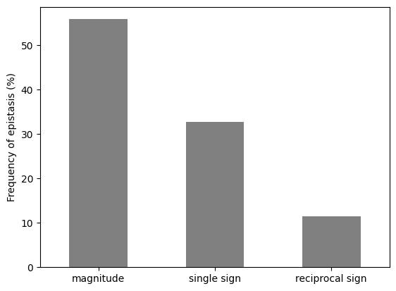
Most squares show only magnitude epistasis, but a third show single sign epistasis and 11% show reciprocal sign epistasis. These proportions agree with those reported by Papkou et al. (about 55%, 33% and 11%).
6.6 Walsh–Hadamard decomposition
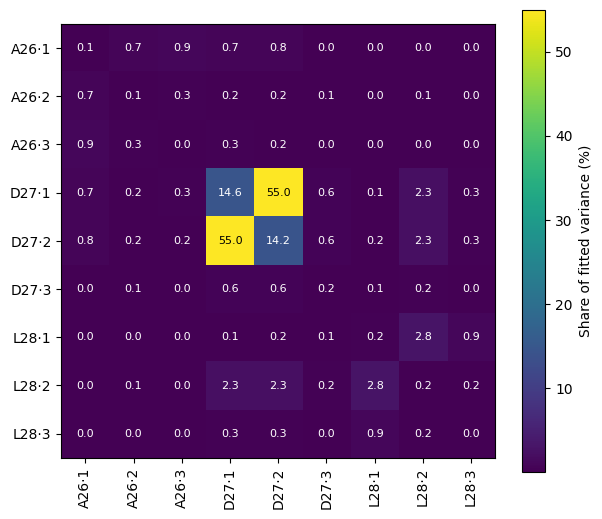
These summaries describe epistasis across the whole landscape, but they do not show which positions are responsible. walsh_hadamard() helps locate it by describing fitness as a sum of single-mutation effects and interactions between pairs of positions, using the multistate extension of Faure et al. (2024). We stop at pairs, leaving higher-order interactions unresolved.
The pairwise model has 352 coefficients, fitted to all 135,178 genotypes by ordinary least squares. Its design matrix has about 48 million entries, above the default max_cells safeguard of 10 million, so we raise that limit explicitly. Compare the first- and second-order training r2; delta_r2 shows the extra variation explained by pairwise terms.
wh = analysis.walsh_hadamard(landscape, max_order=2, max_cells=5e7)
wh["order_summary"]
Output
| order | r2 | delta_r2 | rmse | n_terms | rank | alpha | model_variance_fraction | n_nonzero | |
|---|---|---|---|---|---|---|---|---|---|
| 0 | 0 | 0.000000 | 0.000000 | 0.389962 | 1 | 1 | NaN | 0.000000 | <NA> |
| 1 | 1 | 0.356538 | 0.356538 | 0.312812 | 28 | 28 | NaN | 0.294879 | <NA> |
| 2 | 2 | 0.758929 | 0.402391 | 0.191467 | 352 | 352 | NaN | 0.705121 | <NA> |
Which positions carry this variation? The fitted coefficients let us split the model’s variance, taken over all possible combinations of nucleotides, into a share for each position (diagonal) and for each pair of positions (off-diagonal). The diagonal holds the additive part and the off-diagonal cells the pairwise part; each pair appears twice, and the diagonal plus one triangle add up to 100%. Unlike individual coefficients, these shares do not depend on the reference nucleotide. Positions are labelled by codon and by place within the codon.
As a check, the pairwise shares add up to the order-2 model_variance_fraction in the table above (0.705).
shares = np.zeros((9, 9))
for positions, terms in wh["coefficients"].query("order > 0").groupby("positions"):
    # Each position has three non-reference nucleotides; the reference has zero effect.
    effects = np.pad(terms["coefficient"].to_numpy().reshape((3,) * len(positions)), (1, 0))
    for axis in range(effects.ndim):
        effects = effects - effects.mean(axis=axis, keepdims=True)
    i, j = positions[0] - 1, positions[-1] - 1
    shares[i, j] = shares[j, i] = (effects**2).mean()
shares = 100 * shares / (np.trace(shares) + np.triu(shares, 1).sum())
print(f"Pairwise share of fitted variance: {np.triu(shares, 1).sum():.1f}%")
Output
Pairwise share of fitted variance: 70.5%
labels = ["A26·1", "A26·2", "A26·3", "D27·1", "D27·2", "D27·3", "L28·1", "L28·2", "L28·3"]
fig, ax = plt.subplots(figsize=(7, 6))
image = ax.imshow(shares, cmap="viridis")
ax.set_xticks(range(9), labels, rotation=90)
ax.set_yticks(range(9), labels)
for (i, j), value in np.ndenumerate(shares):
    ax.text(j, i, f"{value:.1f}", ha="center", va="center", fontsize=8,
            color="black" if value > shares.max() / 2 else "white")
fig.colorbar(image, label="Share of fitted variance (%)")
plt.show()
Output
6.7 Diminishing returns and increasing costs
Interactions between particular positions are one source of background dependence. Another is a general trend with how fit the background already is, known as global epistasis. Beneficial mutations can help less in fitter backgrounds, known as diminishing returns (Chou et al., 2011), while deleterious mutations can cost more, known as increasing costs (Johnson et al., 2019).
diminishing_returns_index() correlates background fitness with the gain of each beneficial mutation; a negative value indicates diminishing returns. increasing_costs_index() correlates background fitness with the loss of each deleterious mutation; a positive value indicates increasing costs. Both pool all mutations together and depend on the fitness scale.
returns = analysis.diminishing_returns_index(landscape)
costs = analysis.increasing_costs_index(landscape)
print(f"Diminishing returns index: {returns:.4f}")
print(f"Increasing costs index: {costs:.4f}")
Output
Diminishing returns index: -0.4765
Increasing costs index: 0.4411
6.8 Global optimum accessibility
Ruggedness and epistasis matter for evolution because peaks can trap adaptive walks. global_optima_accessibility() asks whether the fittest variant can still be reached: it returns the fraction of variants from which some path of fitness-increasing single mutations leads to the global optimum. A value of 1 means every variant has such a path; a small value means most adaptive walks must end at other peaks.
accessibility = analysis.global_optima_accessibility(landscape)
print(f"Global optimum accessibility: {accessibility:.4f}")
Output
Global optimum accessibility: 0.7235
6.9 Fitness-distance correlation
Accessibility tells us whether an uphill path to the global optimum exists, not whether fitness points towards it. Jones and Forrest (1995) introduced fitness-distance correlation for this question. fdc() correlates each variant’s fitness with its number of mutations from the global optimum. A negative value means fitter variants tend to lie closer to the best variant; a value near zero means distance tells us little about fitness.
fitness_distance_r = analysis.fdc(landscape, method="spearman")
print(f"Fitness-distance correlation: {fitness_distance_r:.4f}")
Output
Fitness-distance correlation: -0.1397
6.10 Basins of attraction
Global optimum accessibility concerns a single peak, but a landscape has many, and each attracts the adaptive walks that start in its basin of attraction. Following Papkou et al., we define the basin of a peak as all genotypes from which some path of fitness-increasing mutations leads to it. A genotype can reach several peaks, so basins overlap and their sizes do not add up to the number of genotypes.
The accessible_paths property computes the basin size of every peak. get_data(lo_only=True) then returns one row per peak, with the basin size in size_basin_accessible. Here are the five fittest peaks:
landscape.accessible_paths  # computes the basin sizes
peaks = landscape.get_data(lo_only=True)
peaks[["fitness", "size_basin_accessible"]].nlargest(5, "fitness")
Output
| fitness | size_basin_accessible | |
|---|---|---|
| 5071 | 1.395792 | 97804 |
| 66598 | 1.371104 | 98604 |
| 22958 | 1.358285 | 97290 |
| 114118 | 1.356266 | 96224 |
| 35489 | 1.356194 | 98687 |
Do fitter peaks attract more genotypes? We can compare peak fitness with basin size, using a Spearman rank correlation and a scatter plot with one point per peak and a least-squares line:
rho = peaks["fitness"].corr(peaks["size_basin_accessible"], method="spearman")
print(f"Spearman correlation between peak fitness and basin size: {rho:.2f}")
ax = peaks.plot.scatter("fitness", "size_basin_accessible", s=10, alpha=0.6,
                        xlabel="Fitness of peak", ylabel="Basin size")
x = np.array([peaks["fitness"].min(), peaks["fitness"].max()])
ax.plot(x, np.polyval(np.polyfit(peaks["fitness"], peaks["size_basin_accessible"], 1), x), color="C3")
plt.show()
Output
Spearman correlation between peak fitness and basin size: 0.62
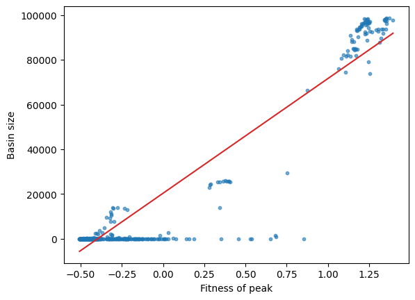
Fitter peaks tend to have larger basins, as Papkou et al. also found. They plotted peaks separately by the amino acid at position 27 (their Fig. S12).
In summary, the DHFR landscape is highly rugged, with 514 peaks and an r/s ratio of 3.36. Sign epistasis is frequent (γ* = 0.142): a third of mutation squares show single sign epistasis and 11% reciprocal sign epistasis. Pairwise terms account for 71% of the fitted variance. More than half of it, 55%, comes from a single pair: the first two nucleotides of codon 27, which together largely determine the encoded amino acid. Beneficial mutations gain less (−0.476) and deleterious mutations cost more (0.441) in fitter backgrounds. Despite this ruggedness, 72.4% of genotypes in the network have a fitness-increasing path to the global optimum, consistent with Papkou et al.’s conclusion that the highest peaks remain accessible through abundant paths. Fitter peaks also tend to have larger basins of attraction (Spearman ρ = 0.62), whereas the median peak attracts only 28 genotypes.
7. Running several analyses together
We can collect the single-value metrics above with analysis.profile(), using the same seed for the idiosyncratic index. landscape.n_lo supplies the peak count directly; the W–H result keeps its separate coefficient and order-summary tables.
analysis.profile(
    landscape,
    metrics=[
        "r_s_ratio", "gamma_star", "global_idiosyncratic_index",
        "diminishing_returns_index", "increasing_costs_index",
        "global_optima_accessibility", "fdc",
    ],
    seed=42, n_jobs=1, progress=False,
)
Output
r_s_ratio                      3.356195
gamma_star                     0.141657
global_idiosyncratic_index     0.459263
diminishing_returns_index     -0.476487
increasing_costs_index         0.441070
global_optima_accessibility    0.723520
fdc                           -0.139723
dtype: float64
8. Analysis reference
For further exploration, analysis.list_metrics() lists the metrics available to profile(). The worked W–H result also exposes fit_info; its order summary separates cumulative training fit from the fitted model’s variance spectrum.
Data sources
Papkou A. et al. (2023). A rugged yet easily navigable fitness landscape. We use the unrounded fitness table fitness_data_wt.rds from the authors’ archive (CC BY 4.0), with columns renamed to sequence and fitness. Its 261,333 genotypes differ from the 261,382 stated in the article.